MACROECONOMICS
Macroeconomics is the study of the economy as a whole, focusing on aggregate variables like:
- National income
- Unemployment rates
- Inflation
- Economic growth
- International trade
Macroeconomics (economy-wide) vs. Microeconomics (individual markets)
Table of Contents
[[#Unit 1 - Basic Economic Concepts]]
- [[#1.1 Scarcity and Opportunity Cost]]
- [[#1.2 Production Possibilities Curve]]
- [[#1.3 Comparative Advantage and Trade]]
[[#Unit 2 - Measuring Economic Performance]]
- [[#2.1 Gross Domestic Product (GDP)]]
- [[#2.2 Unemployment]]
- [[#2.3 Inflation and Price Indices]]
[[#Unit 3 - National Income and Price Determination]]
- [[#3.1 Aggregate Demand (AD)]]
- [[#3.2 Aggregate Supply (AS)]]
- [[#3.3 Macroeconomic Equilibrium]]
[[#Unit 4 - The Financial Sector]]
- [[#4.1 Money and Banking]]
- [[#4.2 The Federal Reserve System]]
- [[#4.3 Monetary Policy]]
- [[#4.4 Money Market and Loanable Funds Market]]
- [[#4.5 Quantity Theory of Money]]
- [[#4.6 Money Supply]]
- [[#4.7 Bank Balance Sheet]]
- [[#4.8 Demand for Money]]
- [[#4.9 Federal Funds Rate and Discount Rate]]
[[#Unit 5 - Inflation, Unemployment, and Stabilization Policies]]
- [[#5.1 The Phillips Curve]]
- [[#5.2 Role of Expectations in Inflation and Unemployment]]
- [[#5.3 Demand-Pull and Cost-Push Inflation]]
- [[#5.4 Stabilization Policies]]
- [[#5.5 The Multiplier Effect]]
[[#Unit 6 - Fiscal Policy and the Role of Government]]
- [[#6.1 Government Spending and Taxation]]
- [[#6.2 Budget Deficits and National Debt]]
- [[#6.3 Fiscal Policy Tools]]
[[#Unit 7 - Economic Growth and Productivity]]
- [[#7.1 Long-Run Economic Growth]]
- [[#7.2 Productivity and Human Capital]]
- [[#7.3 Investment and Capital Stock]]
- [[#7.4 Convergence Hypothesis]]
[[#Unit 8 - International Economics]]
- [[#8.1 Balance of Payments]]
- [[#8.2 Exchange Rates]]
- [[#8.3 Trade Policies]]
[[#Formulas and Charts]]
Unit 1 - Basic Economic Concepts
1.1 Scarcity and Opportunity Cost
Scarcity: Limited resources relative to unlimited wants
- Fundamental economic problem
Opportunity Cost: The value of the next best alternative
1.2 Production Possibilities Curve
Production Possibilities Curve (PPC): Shows the maximum combinations of two goods that can be produced with available resources
Key Concepts:
- Points inside the curve = inefficient (able to produce more of either good with same resources)
- Points on the curve = efficient (no inefficiency)
- Points outside the curve = unattainable (need more or better resources)
Shape: Typically bowed outward (concave) due to increasing opportunity costs
Shifts in PPC:
- Inward shift: Reduced production (depleted resource, regulation)
- Outward shift: Increased production (technology, trade, growth)
1.3 Comparative Advantage and Trade
Absolute Advantage: Ability to produce more of a good with the same resources
Comparative Advantage: Ability to produce a good at a lower opportunity cost
- Countries should specialize in goods where they have comparative advantage
Terms of Trade: Exchange rate between two goods in trade
Unit 2 - Measuring Economic Performance
2.1 Gross Domestic Product (GDP)
GDP: Total market value of all final goods and services produced within a country in a given period
Circular Flow Model
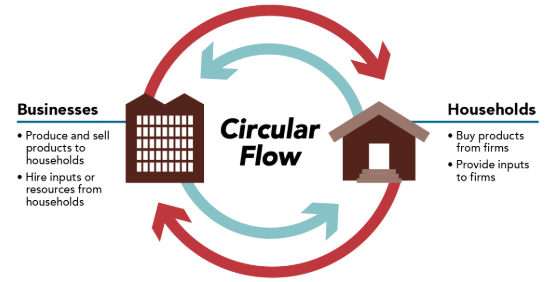
The Circular Flow Model illustrates how money, goods, services, and resources flow continuously between the key sectors of the economy — and why total spending always equals total income equals total output.
Two-Sector Model (Households & Firms):
- Households own all factors of production (labor, land, capital, entrepreneurship) and supply them to firms through the Factor Market in exchange for income (wages, rent, interest, profit)
- Firms use those factors to produce goods and services, then sell them to households through the Product Market in exchange for consumer spending
- The flow is circular: household income → consumer spending → firm revenue → factor payments → household income again
Four-Sector Model (adds Government & Foreign Sector):
- Government: Collects taxes from households and firms (a leakage); injects money back through government spending (G) and transfer payments
- Foreign Sector: Exports add money to the domestic circular flow (an injection); imports drain money out (a leakage); net effect = Net Exports (X − M)
Leakages vs. Injections:
| Leakages (remove $ from flow) | Injections (add $ to flow) |
|---|---|
| Saving (S) | Investment (I) |
| Taxes (T) | Government Spending (G) |
| Imports (M) | Exports (X) |
Key Insight: In equilibrium, total leakages = total injections, and:
Why it matters: The circular flow explains how a disruption in one sector ripples through the whole economy. If households save more (leakage increases), firms receive less revenue, cut production, pay less in wages — income falls. This is why injections (like government spending) are used to stabilize the flow during recessions.
Expenditure Approach: All money spent
= Consumer spending = Investment (business spending on capital goods) = Government spending = Net Exports ( )
Income Approach: All money made
Important Distinctions:
- Real GDP: Adjusted for inflation (constant prices)
- GDP Deflator: Real GDP as a percent of Nominal GDP
Nominal GDP is Current year good times Current year prices
Real GDP is Current years goods times Base year prices
What's NOT Counted in GDP:
- Factors of production
- Financial transactions (stocks, bonds)
- Transfer payments (Social Security, welfare)
- Underground economy
- Non-market activities (household work)
2.2 Unemployment
Labor Force: Employed + Unemployed (actively seeking work)
Unemployment Rate Formula:
Labor Force Participation Rate:
Types of Unemployment
Frictional: Temporary unemployment during job transitions
- Job searching, entering workforce
- Always present in economy
Structural: Skills mismatch with available jobs
- Technological changes, industry shifts
- Long-term unemployment
Cyclical: Due to economic downturns/recessions
- Fluctuates with business cycle
- Target of stabilization policies
Seasonal: Predictable patterns (agriculture, tourism)
Natural Rate of Unemployment (NRU):
- Unemployment rate when economy is at full employment
- Also called Full Employment Rate
- Typically 4-5% in the U.S.
Full Employment: cyclical unemployment = 0 (Economy operating at natural rate)
2.3 Inflation and Price Indices
Inflation: General increase in price level over time
Deflation: General decrease in price level
Disinflation: Decrease in the inflation rate (prices still rising, but more slowly)
Consumer Price Index (CPI):
- Used to measure cost of living
CPI Formula:
Inflation Rate Formula:
Real vs. Nominal Values:
Real Interest Rate:
Effects of Inflation:
- Losers: Savers, lenders, those on fixed incomes
- Menu costs: Cost of changing prices
- Shoe-leather costs: Cost of reducing money holdings
Unit 3 - National Income and Price Determination
3.1 Aggregate Demand (AD)
Aggregate Demand: Total quantity of goods and services demanded at different price levels
AD Curve: Downward sloping
Why AD Slopes Downward:
- Wealth Effect: Lower prices increase real wealth → more spending
- Interest Rate Effect: Higher prices → Higher interest rates (lenders need REAL return) → less investment
- Foreign Trade Effect: Higher domestic prices → less exports, more imports (lower net exports)
Shifts in AD
Increase AD (out):
- Increase in investment spending
- Increase in government spending
- Decrease in taxes
- Increase in exports
- Decrease in imports
- Increase in money supply - highest liquidity money M1
Decrease AD (in):
- Consumer confidence falls
- Higher interest rates
- Decrease in money supply
- Selling bonds (crowding out)
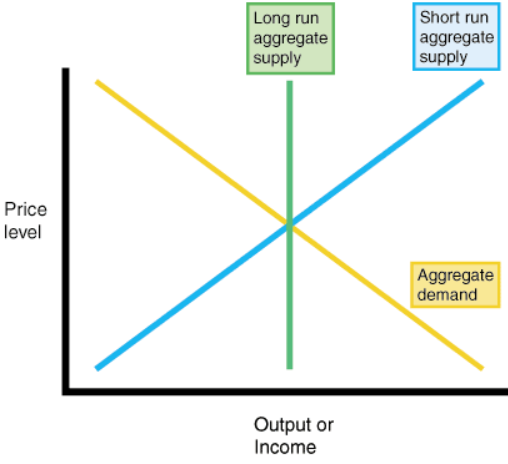
3.2 Aggregate Supply (AS)
Aggregate Supply: Total quantity of goods and services firms produce at different price levels
Short-Run Aggregate Supply (SRAS):
- Upward sloping
- Input prices are sticky/fixed in short run
Long-Run Aggregate Supply (LRAS):
- Economy produces at maximum sustainable level
- Located at Natural Rate of Unemployment
Shifts in SRAS:
- Changes in productivity
- Supply shocks
- Changes in business taxes/regulations
- Future price expectations (lower price expectations increase SRAS)
Shifts in LRAS:
- Changes in technology
- Changes in institutions/regulations
- Changes in human capital
3.3 Macroeconomic Equilibrium
Short-Run Equilibrium: Where AD intersects SRAS
Long-Run Equilibrium: Where AD intersects both SRAS and LRAS
Recessionary Gap:
- Unemployment > Natural rate
- Below full employment
- Real GDP < Potential GDP
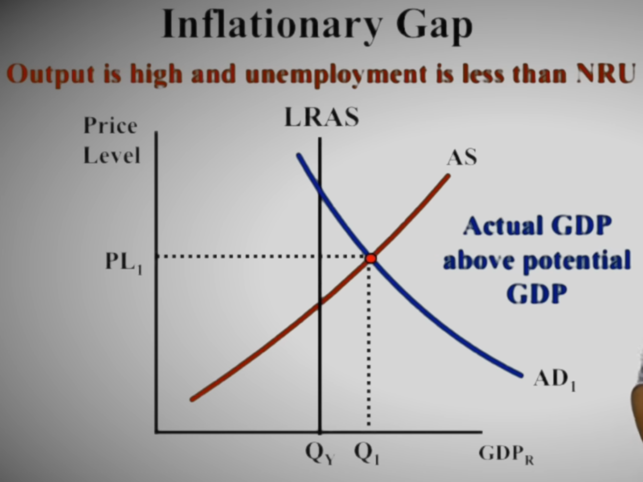
Inflationary Gap:
- Unemployment is lower than natural rate
- Real GDP > Potential GDP
- Inflation is higher than target
- Increased prices and wages will bring AS back to LRAS at a higher price level
Can be caused by an increase in MS (see expansionary monetary policy graph)
Output Gap
The Output Gap measures the difference between an economy's actual output and its potential (full-employment) output.
Negative Output Gap (Recessionary Gap):
- Actual GDP < Potential GDP → economy is underperforming
- Unemployment is above the natural rate
- Unused capacity (workers, factories sitting idle)
- Policy response → Expansionary Fiscal Policy:
- Government increases spending or cuts taxes → AD shifts right
- The spending multiplier amplifies the initial injection, closing the gap
- Example: If the gap is −$500B and the spending multiplier is 5, the government needs to spend $100B to close it
- Graph: AD shifts right until it intersects LRAS at full-employment output
Positive Output Gap (Inflationary Gap):
- Actual GDP > Potential GDP → economy is overheating
- Unemployment is below the natural rate
- Upward pressure on wages and prices
- Policy response → Contractionary Fiscal Policy: increase taxes or cut spending → AD shifts left
Key Link: Expansionary fiscal policy is specifically designed to close a negative output gap. The size of the required policy change depends on the size of the gap divided by the multiplier.
Self-Correction:
- Recessionary gap → wages fall → SRAS shifts right
- Inflationary gap → wages rise → SRAS shifts left
Unit 4 - The Financial Sector
4.1 Money and Banking
Functions of Money:
- Medium of Exchange: Facilitates transactions
- Unit of Account: Measure of value
- Store of Value: Maintains purchasing power over time
Time Value of Money:
- Present Value: Current value
- Future Value: Value after interest
-
4.2 The Federal Reserve System
The Fed: Central bank of the United States
Structure:
- 12 Regional Federal Reserve Banks
- Federal Open Market Committee (FOMC)
Functions of the Fed:
- Conduct monetary policy
- Supervise and regulate banks
- Maintain financial system stability
- Provide banking services to government and banks
FOMC: Makes monetary policy decisions
- Controls money supply and interest rates
4.3 Monetary Policy
Monetary Policy: Fed's actions to influence money supply and interest rates
Goals:
- Full employment
- Economic growth
- Price Stability (limit inflation)
Tools of Monetary Policy
Open Market Operations (OMO): Most common tool
- Buying bonds: Expansionary — Money enters economy → Increases money supply → lowers interest rates
- Selling bonds: Contractionary — Money leaves economy → Decreases money supply → raises interest rates
Discount Rate: Interest rate the Fed charges commercial banks for short-term loans from the Fed's "discount window"
- Lower discount rate: Expansionary — banks borrow more cheaply from the Fed → lend more → money supply grows
- Higher discount rate: Contractionary — borrowing from the Fed becomes expensive → banks lend less → money supply shrinks
- The discount rate signals the Fed's monetary policy stance
- Banks prefer borrowing from each other (federal funds market) before going to the discount window, so the discount rate typically sits above the federal funds rate
- See [[#4.9 Federal Funds Rate and Discount Rate]] for a detailed comparison
Reserve Requirement: Percentage of deposits banks must hold
- Lower requirement: Expansionary (more lending)
- Higher requirement: Contractionary (less lending)
Money Multiplier:
Change in Money Supply:
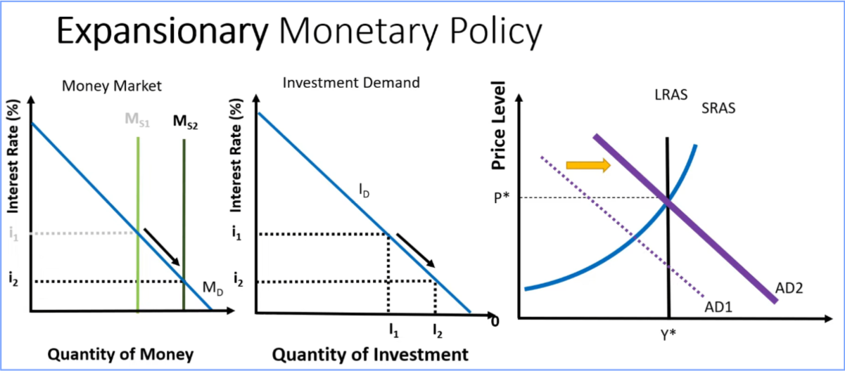
Expansionary Monetary Policy (Easy Money):
- Buying bonds (liquidizing)
- Stimulate spending and investment
- Used during recessions
- Effect: AD shifts right
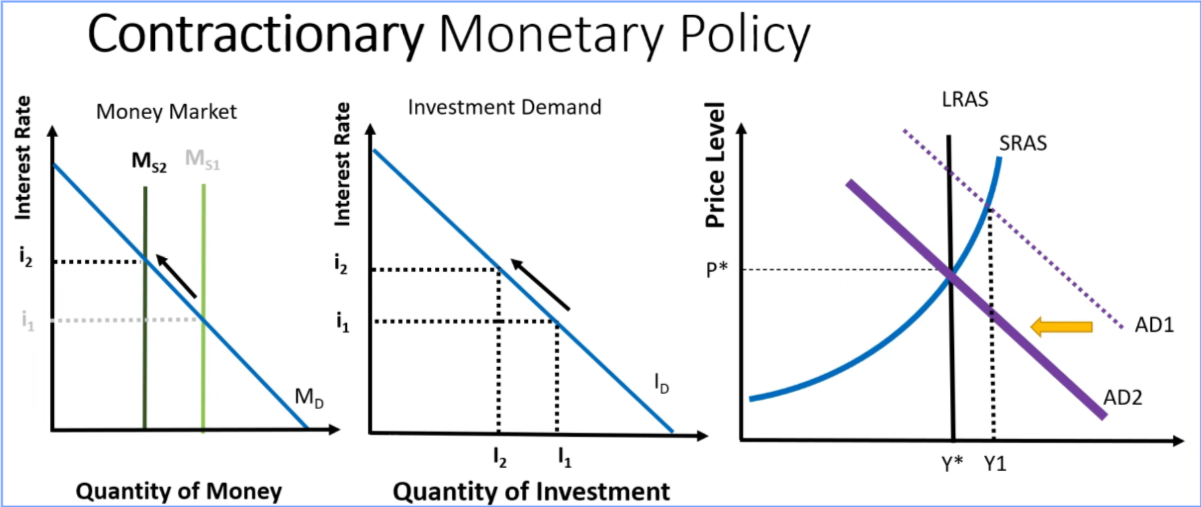
Contractionary Monetary Policy (Tight Money):
- Raise interest rates
- Reduce spending and investment
- Used during inflation
- Effect: AD shifts left
Monetary Policy Transmission:
- Fed changes money supply
- Interest rates change
- Investment spending changes
- AD shifts
- Real GDP and price level change
4.4 Money Market and Loanable Funds Market
Money Market
The Money Market shows how the nominal interest rate is determined by the supply and demand for money.
Money Demand (Md):
- Downward sloping — lower interest rates → people hold more money (less incentive to hold bonds)
- Shifts right (increases): Higher price level, higher real GDP, increased transactions
- Shifts left (decreases): Lower price level, lower real GDP, improved payment technology
Money Supply (Ms):
- Vertical — controlled by the Fed, independent of interest rate
- Shifts right: Fed buys bonds (expansionary), lower reserve requirement, lower discount rate
- Shifts left: Fed sells bonds (contractionary), higher reserve requirement, higher discount rate
Equilibrium: Where Md = Ms → determines the nominal interest rate
Policy Effects:
- Fed increases Ms → Ms shifts right → nominal interest rate falls → investment increases → AD shifts right
- Fed decreases Ms → Ms shifts left → nominal interest rate rises → investment decreases → AD shifts left
Loanable Funds Market
The Loanable Funds Market shows how the real interest rate is determined by the supply and demand for savings/loans.
Demand for Loanable Funds:
- Downward sloping — lower real interest rates → more borrowing for investment
- Shifts right: Business optimism, new investment opportunities, government borrowing (deficit spending)
Supply of Loanable Funds:
- Upward sloping — higher real interest rates → more saving
- Shifts right: Increased household saving, capital inflows from abroad, higher disposable income
- Shifts left: Decreased saving, increased government budget deficit
Equilibrium: Where supply = demand → determines the real interest rate
Crowding Out (revisited in the loanable funds context):
- Government borrows more → demand for loanable funds shifts right → real interest rate rises → private investment falls
Key Distinction:
| Money Market | Loanable Funds Market | |
|---|---|---|
| Variable | Nominal interest rate | Real interest rate |
| Supply controlled by | The Fed | Savers / households |
| Demand driven by | Liquidity preference | Investment demand |
Limitations of Monetary Policy:
- Time lags: Recognition, implementation, impact lags
- Inflation expectations: Can undermine policy effectiveness
4.5 Quantity Theory of Money
The Quantity Theory of Money explains the long-run relationship between money supply and the price level.
The Equation of Exchange:
= Money supply = Velocity of money (average number of times a dollar is spent per year) = Price level = Real output (real GDP) - Note:
= Nominal GDP
Key Assumptions:
(velocity) is relatively stable in the long run (real output) is determined by real factors (resources, technology) — independent of money supply in the long run
Conclusion: In the long run, increases in the money supply lead to proportional increases in the price level (inflation), not real output.
Policy Implication: If the Fed doubles the money supply, the price level approximately doubles in the long run. This is the basis for the classical view that "inflation is always and everywhere a monetary phenomenon."
Short Run vs. Long Run:
- Short run: Increases in M can raise both P and Y (real output)
- Long run: Increases in M primarily raise P; Y returns to potential
Connecting to AD-AS: An increase in M → AD shifts right → in the short run, both P and Y rise; in the long run, only P rises as Y returns to potential GDP (LRAS).
Exam tip: If V and Y are held constant, the equation becomes a direct relationship: more money = higher prices. The Fed uses this logic when warning that excessive money creation causes inflation.
4.6 Money Supply
The money supply refers to the total amount of money in circulation in an economy. The Fed tracks it using different measures based on liquidity (how easily an asset can be used as cash).
| Measure | What's Included | Liquidity |
|---|---|---|
| M0 | Physical currency (coins and paper bills) | Highest |
| M1 | M0 + demand deposits (checking accounts) + traveler's checks | High |
| M2 | M1 + savings accounts + money market accounts + small CDs | Lower |
Key point: M1 is the most liquid and is most directly controlled by the Fed. M2 is broader and used more for long-run inflation analysis.
How the Fed Changes the Money Supply:
| Action | Effect on Money Supply |
|---|---|
| Buy bonds (OMO) | Increases (expansionary) |
| Sell bonds (OMO) | Decreases (contractionary) |
| Lower reserve requirement | Increases (banks lend more) |
| Raise reserve requirement | Decreases (banks lend less) |
| Lower discount rate | Increases (cheaper to borrow from Fed) |
| Raise discount rate | Decreases (more expensive to borrow from Fed) |
Money Creation Process:
- When a bank receives a deposit, it keeps a fraction in reserve and lends the rest
- That loan becomes a deposit at another bank, which lends again
- Each round creates new money → this is the money multiplier in action
Example: $1,000 deposit with a 10% reserve requirement:
4.7 Bank Balance Sheet
A bank balance sheet shows what a bank owns (assets) and what it owes (liabilities), plus the owners' equity. It must always balance:
T-Account Structure
| Assets | Liabilities + Equity |
|---|---|
| Required Reserves | Deposits (demand + time) |
| Excess Reserves | Borrowings (from Fed or other banks) |
| Loans | |
| Securities (bonds) | Equity |
| Physical assets | Owners' equity (net worth) |
Key Terms:
-
Required Reserves: Minimum amount the bank must hold (set by the Fed's reserve requirement ratio)
-
Excess Reserves: Any reserves held above the required minimum
- Excess reserves represent the bank's lending capacity — this is the amount that can be loaned out and enter the money supply
-
Loans: The primary way banks earn income (interest payments from borrowers)
Reading a T-Account Example:
| Assets | Liabilities | ||
|---|---|---|---|
| Reserves | $200 | Deposits | $1,000 |
| Loans | $800 | ||
| Total | $1,000 | Total | $1,000 |
With a 10% reserve requirement:
- Required reserves = $1,000 × 0.10 = $100
- Excess reserves = $200 − $100 = $100 (can still lend this out)
Balance Sheet Changes from Fed Actions:
| Fed Action | Bank Asset Change | Effect |
|---|---|---|
| Fed buys bonds from bank | Bonds ↓, Reserves ↑ | More excess reserves → more lending |
| Fed sells bonds to bank | Bonds ↑, Reserves ↓ | Fewer excess reserves → less lending |
| New deposit arrives | Reserves ↑ | Money multiplier process begins |
Exam tip: On the CLEP, you may be given a T-account and asked how much a bank can lend. The answer is always the excess reserves, not the total reserves.
4.8 Demand for Money
The demand for money refers to how much of their wealth people want to hold in liquid form (cash and checking accounts) rather than in interest-bearing assets like bonds.
There are two main reasons people demand money:
Transaction Demand
- People hold money to pay for everyday purchases — groceries, bills, rent
- Driven by income and spending levels: higher income → more transactions → more money needed
- Relatively insensitive to interest rates — you need cash to buy things regardless of what interest rates are doing
- Increases with: higher real GDP, higher price level (more nominal spending needed)
Asset (Speculative) Demand
- People hold money as a store of value or safe asset instead of riskier alternatives
- When interest rates are high, bonds and savings accounts pay well → people hold less money (opportunity cost of holding cash is high)
- When interest rates are low, the opportunity cost of holding cash falls → people prefer holding more money
- This is why the money demand curve slopes downward — as interest rates fall, quantity of money demanded rises
The Money Demand Curve
| Factor | Effect on Money Demand Curve |
|---|---|
| Higher real GDP / income | Shifts right (more transactions needed) |
| Higher price level | Shifts right (same purchases cost more) |
| Higher interest rates | Move along the curve (decrease quantity demanded) |
| Improved payment technology (e.g., credit cards, digital wallets) | Shifts left (less cash needed for transactions) |
Key distinction: Changes in income or price level shift the demand curve. Changes in the interest rate cause movement along the curve.
Money Market Equilibrium:
- The intersection of money demand (downward sloping) and money supply (vertical, set by the Fed) determines the nominal interest rate
- If the Fed increases the money supply (shifts Ms right) → interest rate falls
- If income rises (shifts Md right) → interest rate rises
4.9 Federal Funds Rate and Discount Rate
These are the two key short-term interest rates in the U.S. banking system, and they are often confused on the CLEP.
Federal Funds Rate
- The interest rate at which commercial banks lend reserves to each other overnight
- Banks with excess reserves lend to banks that are short of reserves
- Set indirectly by the Fed through open market operations — the Fed does not directly set this rate, but targets it by adjusting the money supply
- The FOMC announces a target range for the federal funds rate at each meeting
- This is the most widely watched interest rate in the economy
How the Fed influences it:
- Fed buys bonds → injects reserves → banks have more to lend to each other → federal funds rate falls
- Fed sells bonds → drains reserves → banks have less to lend → federal funds rate rises
Discount Rate
- The interest rate the Fed charges commercial banks that borrow directly from the Fed (through the "discount window")
- Set directly by the Fed (unlike the federal funds rate)
- Typically set above the federal funds rate — borrowing from the Fed is a last resort
- Banks prefer to borrow from each other (federal funds market) before going to the Fed
How it works:
- Lower discount rate → cheaper for banks to borrow from the Fed → banks more willing to lend → money supply increases → expansionary
- Higher discount rate → more expensive to borrow from the Fed → banks lend less → money supply decreases → contractionary
Side-by-Side Comparison
| Feature | Federal Funds Rate | Discount Rate |
|---|---|---|
| Who lends? | One commercial bank to another | The Fed to commercial banks |
| Set by | Market forces (influenced by Fed OMO) | The Fed directly |
| Typical level | Lower | Higher (penalty rate) |
| Signals | General market conditions | Fed's official policy stance |
| Most common tool? | Yes — most commonly watched rate | No — used as a backup/signal |
Exam tip: When the Fed lowers the discount rate, it becomes cheaper for banks to borrow from the Fed → more money in the banking system → lower interest rates economy-wide → expansionary effect. When it raises the discount rate, the opposite occurs.
Unit 5 - Inflation, Unemployment, and Stabilization Policies
5.1 The Phillips Curve
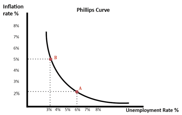
Phillips Curve: Shows inverse relationship between inflation and unemployment
Short-Run Phillips Curve (SRPC):
- Trade-off between inflation and unemployment
- Can shift due to supply shocks or changes in expectations
Changes in AS/AD will cause changes in the SR Phillips curve
- Movement along AS (Shift in AD) will cause a mirrored Movement in SRPC
- Shift of AS (Movement of AD) will cause a mirrored Shift in SRPC
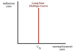
Long-Run Phillips Curve (LRPC):
- No long-run trade-off between inflation and unemployment
- Unemployment returns to natural rate regardless of inflation
Short-Run Phillips Curve (SRPC) — Shifts: Causes and Effects
The SRPC can shift, meaning the entire trade-off changes — different combinations of inflation and unemployment become possible at every point.
What causes the SRPC to shift RIGHT (stagflation — worse trade-off)?
| Cause | Mechanism |
|---|---|
| Negative supply shock (e.g., oil price spike) | Production costs rise → SRAS shifts left → higher prices AND higher unemployment simultaneously |
| Higher inflation expectations | Workers demand higher wages anticipating inflation → costs rise → SRPC shifts right |
| Increased input costs (wages, raw materials) | Same effect as a supply shock → higher costs at every output level |
- A rightward SRPC shift means: for any unemployment rate, inflation is now higher → stagflation
- AD-AS link: A leftward shift in SRAS corresponds to a rightward shift in the SRPC
What causes the SRPC to shift LEFT (favorable trade-off)?
| Cause | Mechanism |
|---|---|
| Positive supply shock (e.g., oil price drop, tech improvement) | Production costs fall → SRAS shifts right → lower inflation and lower unemployment |
| Lower inflation expectations | Workers accept lower wages → costs fall → SRPC shifts left |
| Increase in productivity | More output per worker → lower cost per unit → lower inflation at each unemployment level |
- A leftward SRPC shift means: for any unemployment rate, inflation is now lower → best of both worlds
Movement along the SRPC (not a shift) is caused by changes in Aggregate Demand:
- AD increases → unemployment falls, inflation rises → move up and left along the curve
- AD decreases → unemployment rises, inflation falls → move down and right along the curve
Key exam distinction: Supply shocks and expectation changes shift the SRPC. Changes in spending (fiscal/monetary policy) cause movement along the existing SRPC.
Movement Along SRPC: Changes in AD
5.2 Role of Expectations in Inflation and Unemployment
Expectations play a central role in shifting the Short-Run Phillips Curve (SRPC) and the Short-Run Aggregate Supply curve (SRAS).
Adaptive Expectations
- People form expectations about future inflation based on past inflation
- If inflation has been high, workers demand higher wages expecting it to continue
- Higher expected inflation → workers and firms build it into wages and prices → SRPC shifts right (upward)
- Implication: Expansionary policy that raises inflation will eventually shift SRPC right, eroding the short-run trade-off
Rational Expectations
- People use all available information (not just past data) to forecast inflation
- If people anticipate a policy change, they adjust immediately — the short-run trade-off may disappear
- Implication: Announced, credible policy changes can affect expectations without going through the short-run output/unemployment process
Expectations and the Phillips Curve
- Short-run: Unexpected inflation can temporarily reduce unemployment (workers accept jobs based on nominal wages; real wages are actually lower)
- Long-run: Once expectations adjust, unemployment returns to the natural rate regardless of inflation
- A positive supply shock or lower inflation expectations → SRPC shifts left (lower inflation at every unemployment level)
- A negative supply shock or higher inflation expectations → SRPC shifts right (stagflation)
Expected vs. Actual Inflation:
- If actual inflation > expected inflation → unemployment falls below natural rate (short run)
- If actual inflation = expected inflation → unemployment equals natural rate (long run)
- Policy credibility matters: Central banks that are trusted to fight inflation can keep expectations anchored low
5.3 Demand-Pull and Cost-Push Inflation
Think about basic supply and demand model
Demand-Pull Inflation:
- Caused by increase in AD without an increase in AS
- Graph: AD shifts right
- Unemployment falls below natural rate (short run)
Cost-Push Inflation:
- Caused by a decrease in SRAS (a negative supply shock) — not caused by an increase in AD
- Results from rising production costs hitting the supply side of the economy
- Graph: SRAS shifts left → price level rises AND real GDP falls simultaneously
- Unemployment rises (stagflation) — distinguishing feature from demand-pull
Common causes of cost-push inflation:
- Rising input costs: Oil price spikes, commodity shortages, rising raw material prices
- Wage increases that outpace productivity (e.g., from minimum wage laws or union contracts)
- Supply disruptions: Natural disasters, pandemics, geopolitical shocks that cut off production
- Government regulations that raise the cost of production
Why it creates a policy dilemma:
- If the Fed tightens to fight inflation → unemployment rises further
- If the Fed loosens to fight unemployment → inflation worsens
- There is no easy fix — policymakers must choose which problem to address first
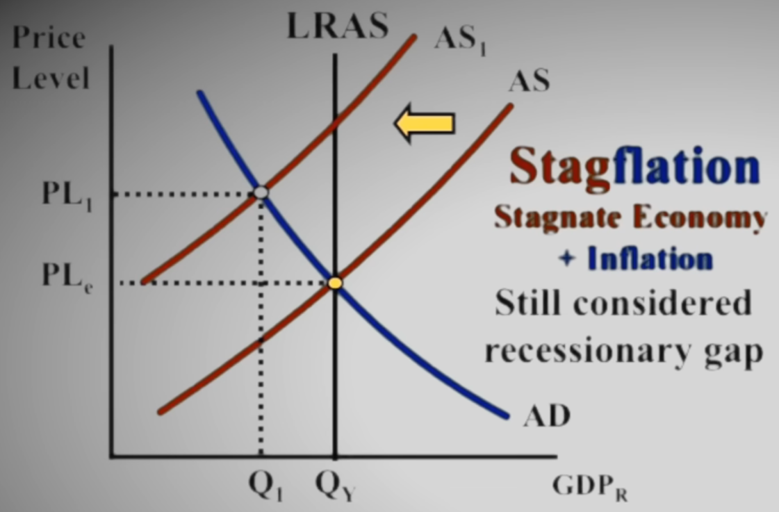
Stagflation = Cost-Push Inflation + High Unemployment: This is the signature outcome of a SRAS leftward shift. It breaks the normal Phillips Curve trade-off and is associated with 1970s-style oil shocks.
Stagflation: High inflation + High unemployment + Low growth
- Creates policy dilemma
5.5 The Multiplier Effect
The Multiplier Effect describes how an initial change in spending leads to a larger overall change in GDP.
Intuition: When the government spends $100, the recipient earns $100 and spends a portion of it; that spending becomes someone else's income, and so on — each round amplifies the original injection.
Marginal Propensity to Consume (MPC): Fraction of additional income that is spent
Marginal Propensity to Save (MPS): Fraction of additional income that is saved
Spending Multiplier
How it works step-by-step:
- Government spends $1,000 → someone earns $1,000
- That person spends $800 (if MPC = 0.8), saves $200
- The $800 becomes income for others → they spend $640, save $160
- Each round adds less and less until the total sums to $5,000
The multiplier is larger when:
- MPC is high (people spend a large fraction of income)
- MPS is low (people save little)
Tax Multiplier
Why the tax multiplier is smaller than the spending multiplier:
- A tax cut of $1,000 does not inject $1,000 directly — households save part of it first
- With MPC = 0.8: the first round of spending is only $800 (not $1,000), so the multiplier effect is smaller
- The tax multiplier is always one less (in absolute value) than the spending multiplier
- The negative sign reflects: tax increases reduce GDP, tax cuts increase GDP
Example with MPC = 0.8:
- $200B increase in government spending → GDP rises by $1,000B
- $200B tax cut → GDP rises by $800B (smaller effect)
Balanced Budget Multiplier: When government increases spending AND taxes by the same amount, the net multiplier = 1 (GDP rises by exactly the spending increase)
Crowding-Out Effect (limits the multiplier):
- Expansionary fiscal policy → government borrows more → real interest rates rise → private investment falls
- Offsets some of the multiplier effect
Factors That Reduce the Multiplier:
- High MPS (people save more of income)
- Crowding out from borrowing
- Imports (spending leaks abroad)
- Taxes (reduce disposable income)
5.4 Stabilization Policies
Goals:
- Higher employment
- Stable prices
- Economic growth
- Stable output
Policy Options:
For Recession (low output, high unemployment):
- Expansionary monetary: Increase money supply, lower interest rates
For Inflation (high prices, economy overheating):
- Contractionary monetary: Decrease money supply, raise interest rates
Policy Coordination:
- Conflicts can arise between Fed and government
Supply-Side Policies: Focus on increasing LRAS
- Deregulation
- Education and training
- Infrastructure investment
- Long-run focus rather than short-run stabilization
Unit 6 - Fiscal Policy and the Role of Government
6.1 Government Spending and Taxation
Fiscal Policy: Government's use of spending and taxation to influence the economy
Discretionary Fiscal Policy: Deliberate changes by Congress
Automatic Stabilizers: Built-in features that automatically adjust
- Unemployment insurance
- Welfare programs
Government Spending:
- Goods and services (defense, infrastructure)
- Interest on debt
Taxation:
- Proportional tax: Same rate regardless of income (flat tax)
- Regressive tax: Tax rate decreases as income increases
6.2 Budget Deficits and National Debt
Budget Deficit: Government spending > Tax revenue in one year
Budget Surplus: Tax revenue > Government spending
Balanced Budget: Spending = Revenue
National Debt: Accumulated deficits over time
Crowding Out Effect:
- Reduces private investment
- Limits effectiveness of expansionary fiscal policy
6.3 Fiscal Policy Tools
Expansionary Fiscal Policy:
- Used during recessions
- Increases AD
- Decrease taxes or increase spending
- Effect: AD shifts right → higher GDP, higher prices
Contractionary Fiscal Policy:
- Used during inflation
- Decreases AD
- Increase taxes or decrease spending
- Effect: AD shifts left → lower GDP, lower prices
Spending Multiplier:
Or:
Tax Multiplier:
Where:
- MPS = Marginal Propensity to Save (percent saving)
- MPC = Marginal Propensity to Consume (percent spending)
Change in GDP:
Limitations of Fiscal Policy:
- Crowding out: Reduces private investment
- Political constraints: Difficult to raise taxes or cut spending
- Increases national debt
Unit 7 - Economic Growth and Productivity
7.1 Long-Run Economic Growth
Economic Growth: Increase in potential GDP over time
- Sustained increase in living standards
Sources of Economic Growth:
- Increase in resources (labor, capital, natural resources)
- Technological progress
- Improved human capital
- Better institutions
7.2 Productivity and Human Capital
Productivity: Output per unit of input (usually per worker or per hour)
Determinants of Productivity:
- Human capital per worker
- Natural resources per worker
- Technological knowledge
Human Capital: Knowledge and skills workers acquire
- Training
- Experience
Increasing Productivity:
- Education and training
- Research and development
- Technological innovation
7.3 Investment and Capital Stock
Investment: Spending on capital goods
- Key driver of long-run growth
Capital Deepening: Increase in capital per worker
- Shifts LRAS right
Relationship Between Investment and Interest Rates:
- Lower interest rates → Higher investment
Crowding Out: Government borrowing raises interest rates
- Can slow long-run growth
7.4 Convergence Hypothesis
The Convergence Hypothesis (also called catch-up effect) proposes that poorer economies tend to grow faster than richer ones, and over time their per capita incomes converge toward those of wealthy nations.
Core Logic:
- Developed countries already have large capital stocks → each additional unit of capital adds less to output (diminishing returns to capital)
- Developing countries have small capital stocks → each new unit of capital is highly productive (high marginal return)
- Result: poorer countries get a bigger "bang" from investment → faster growth rates → gradual catch-up
Two Types of Convergence:
| Type | Meaning |
|---|---|
| Absolute Convergence | All countries eventually reach the same income level regardless of starting point |
| Conditional Convergence | Countries converge to their own steady state, which depends on institutions, policies, and savings rates — countries with similar characteristics converge to each other |
Conditions that accelerate convergence:
- Open trade and foreign investment (technology and capital flow to poor countries)
- Strong institutions (rule of law, property rights, low corruption)
- High savings and investment rates
- Education and human capital development
- Political stability
Evidence and Limitations:
- Conditional convergence has strong empirical support — countries with similar institutions do converge
- Absolute convergence is weaker — some countries remain persistently poor due to institutional failures, conflict, or lack of investment
- The technology gap matters: developing countries can adopt existing technology cheaply rather than inventing it, which accelerates growth
Exam tip: Convergence does not mean all countries become equally rich automatically. It means that, all else equal, poorer countries have the potential to grow faster. Poor institutions, political instability, and lack of investment can block convergence entirely.
Connection to the PPC: A developing country's PPC shifts outward faster than a rich country's when it adopts existing technology or attracts capital investment — the same mechanism as convergence.
Unit 8 - International Economics
8.1 Balance of Payments
| Account | Components |
|---|---|
| Current (Trade) Account | Goods, Services, Money, Remittances |
| Capital (Financial) Account | Assets |
- Surplus means a higher inflows
- Deficit means a higher outflows
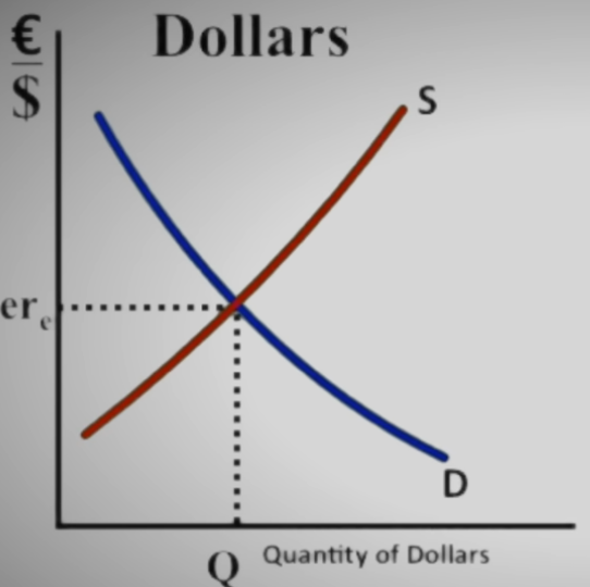
8.2 Exchange Rates
Exchange Rate: Price of one currency in terms of another
- Set by the Supply and Demand for each currency
Appreciation: Currency increases in value relative to another
- Domestic goods become more expensive for foreigners → exports fall
- Foreign goods become cheaper domestically → imports rise
- Net exports decrease → AD decreases
Depreciation: Currency decreases in value relative to another
- Domestic goods become cheaper for foreigners → exports rise
- Foreign goods become more expensive domestically → imports fall
- Net exports increase → AD increases
Causes of Currency Appreciation
A currency appreciates when demand for it rises or supply of it falls:
| Cause | Why it appreciates |
|---|---|
| Higher domestic interest rates | Foreign investors buy domestic bonds → need domestic currency → demand rises |
| Lower domestic inflation | Domestic goods stay competitive → less importing → less currency supplied |
| Increased preference for domestic goods | Foreigners buy more exports → need more domestic currency |
| Political/economic stability | Safe-haven demand → capital flows in |
| Trade surplus | More exports = more foreign currency exchanged for domestic → demand rises |
Causes of Currency Depreciation
A currency depreciates when demand for it falls or supply of it rises:
| Cause | Why it depreciates |
|---|---|
| Lower domestic interest rates | Less attractive to foreign investors → capital flows out |
| Higher domestic inflation | Domestic goods less competitive → more imports → more currency supplied |
| Higher domestic income | More imports consumed → more domestic currency sold for foreign → supply rises |
| Decreased preference for domestic goods | Fewer exports → less demand for domestic currency |
| Political/economic instability | Capital flight → domestic currency sold |
Acronym to remember causes of exchange rate shifts — PIER:
- Preferences (for domestic vs. foreign goods)
- Inflation (relative inflation rates)
- Earnings/Income (relative income levels)
- Returns (interest rates/investment returns)
Exchange Rate Systems:
- Fixed: Government maintains rate
- Managed float: Mostly market with some intervention
Real Exchange Rate: Adjusted for price level differences
8.3 Trade Policies
Free Trade: No restrictions on international trade
- Based on comparative advantage
- Can harm some industries/workers
Protectionism: Policies restricting trade
Trade Barriers
Tariffs: Taxes on imports
- Raises domestic price
- Reduces quantity imported
- Creates deadweight loss
Quotas: Limits on quantity imported
- Similar effects to tariffs
- May be more restrictive
Subsidies: Government payments to domestic producers
- Helps domestic industry compete
Non-tariff barriers: Regulations, standards
- Can restrict trade without obvious barriers
Arguments for Protection:
- National security
- Protect jobs
- Prevent dumping
Arguments Against Protection:
- Higher prices for consumers
- Invites retaliation
- Rent-seeking behavior
Formulas and Charts
Write formulas and draw charts on scratch paper before starting the test
GDP
DOES NOT include: Intermediate good, nonproduction (stocks etc...), non-market goods
Expenditure Approach
- Consumption
- Investment
- Government spending
- Net Exports
Same as aggregate demand
Income Approach
- Wages
- Rent
- Interest
- Profit
Real GDP =
GDP Deflator =
- Nominal GDP
- Real GDP
Employment and Inflation
Unemployment Rate =
Participation Rate =
Inflation
- Consumer Price Index
- Price of Market Basket
Quantity Theory of Money
- Money Supply
- Velocity (average times a dollar is exchanged yearly)
- Price Level
- Output Quantity
Multiplier Effect
Spending Multiplier =
Tax Multiplier =
Marginal Propensity to Save
- Change in Spending
- Change in Income
Marginal Propensity to Consume
- Change in Consumption
- Change in Income
Money Multiplier
- Same concept as spending multiplier with banks as "lenders"
- This gives the amount of NEW loans, or new money added
- For total deposits, you add the original deposit
- For new loans, you do not add the original deposit
Net Capital Outflow
- Money Flows
- Investment Income
- Net Exports
Formulas and Charts
Charts
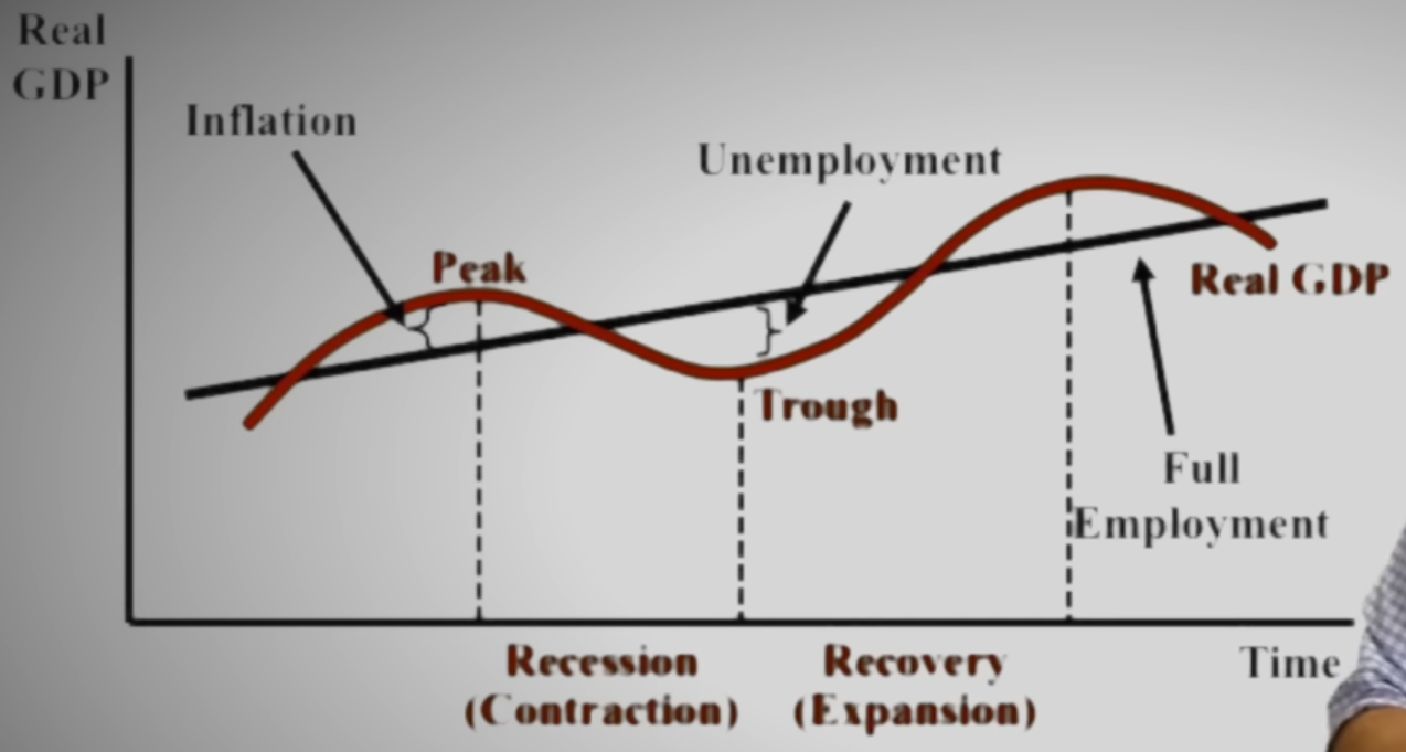
Business Cycle
Stagflation
Inflationary Gap
Phillips Curve
Monetary Policy
Expansionary
Contractionary
| Policy | Tool | Effect on MS | Effect on Interest Rates | Effect on AD |
|---|---|---|---|---|
| Expansionary Monetary | Buy bonds | ↑ | ↓ | ↑ Right |
| Contractionary Monetary | Sell bonds | ↓ | ↑ | ↓ Left |
| Expansionary Fiscal | ↑ Spending | — | ↑ (Crowding out) | ↑ Right |
| Contractionary Fiscal | ↓ Spending | — | ↓ (Crowding out) | ↓ Left |
Exchange Rate
- X: Quantity, Y: Relative Value
- Exchange Rate is the Equilibrium
- Shifts: with a change in Demand, the other must Supply
- (Increased demand means the other increases supply)